I stumbled upon a great
post about adding GIFs to
plots using the Magick package. Curious, I thought I’d give it a shot as well. As I jammed out to Demon Days, arguably the Gorillaz’s best album, the answer of what to visualize was obvious. I would pay homage
to the virtual band’s early hit, Feel Good Inc, by looking at the
positivity of each track.
Gorillaz is a British virtual band created by musician Damon Albarn and artist Jamie Hewlett. The band consists of four animated members:
Murdoc Niccals, Russel Hobbs, Noodle, and 2-D

To get the data regarding the valence (song positivity), I used
spotifyr to pull the audio
features
of each track. I filtered out any live albums.
spotifyris an useful wrapper for pulling audio track features from Spotify’s Web API in bulk. Requires setting up a Dev account with Spotify and linking to spotifyr in R.Valence: A measure from 0.0 to 1.0 describing the musical positiveness conveyed by a track. Tracks with high valence sound more positive (e.g. happy, cheerful, euphoric), while tracks with low valence sound more negative (e.g. sad, depressed, angry).
library(spotifyr)
library(tidyverse)

gorillaz <- get_artist_audio_features('Gorillaz')
gorillaz <- gorillaz %>%
  select(track_name, album_name, valence, album_release_year) %>%
  filter(album_name != "Demon Days Live At The Manchester Opera House")

album_names <- gorillaz %>%
  arrange(album_release_year) %>%
  mutate(label = paste0(album_name, " (", year(album_release_year), ")")) %>%
  pull(label) %>% unique

library(knitr)
kable(head(gorillaz, 10), row.names = F, align='l')
| track_name | album_name | valence | album_release_year |
|---|---|---|---|
| Re-Hash | Gorillaz | 0.782 | 2001-03-26 |
| 5/4 | Gorillaz | 0.805 | 2001-03-26 |
| Tomorrow Comes Today | Gorillaz | 0.561 | 2001-03-26 |
| New Genius (Brother) | Gorillaz | 0.497 | 2001-03-26 |
| Clint Eastwood | Gorillaz | 0.524 | 2001-03-26 |
| Man Research (Clapper) | Gorillaz | 0.838 | 2001-03-26 |
| Punk | Gorillaz | 0.519 | 2001-03-26 |
| Sound Check (Gravity) | Gorillaz | 0.420 | 2001-03-26 |
| Double Bass | Gorillaz | 0.569 | 2001-03-26 |
| Rock the House | Gorillaz | 0.612 | 2001-03-26 |
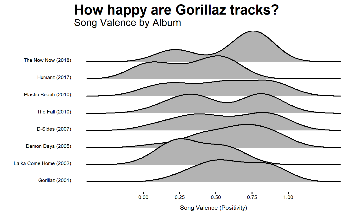
Now that we have the data for all the Gorillaz tracks, we can create a ridgeplot to show the valence distributions by album ordered by release date. This will serve as the background of our GIF project.
library(ggridges)
library(lubridate)

ggplot(gorillaz, aes(x = valence, y = as.character(album_release_year))) +
  geom_density_ridges() +
  theme_ridges(center_axis_labels = TRUE, grid = FALSE, font_size = 6) +
  labs(x = "Song Valence (Positivity)", y = "") +
  ggtitle("How happy are Gorillaz tracks?", "Song Valence by Album") +
  scale_x_continuous(breaks = c(0,0.25, 0.5, 0.75, 1)) +
  scale_y_discrete(labels = album_names) +
  theme(plot.title = element_text(face = 'bold', size = 14, hjust = 0),
        plot.subtitle = element_text(size = 10, hjust = 0))

Now let’s load the gif using the
Magick
package. I had to make sure the background was transparent, and the
frames were not stacked.
library(magick)

plot_gif <- image_read('Gorillaz gif.gif')
plot_gif <- image_scale(plot_gif, "250")
plot_gif

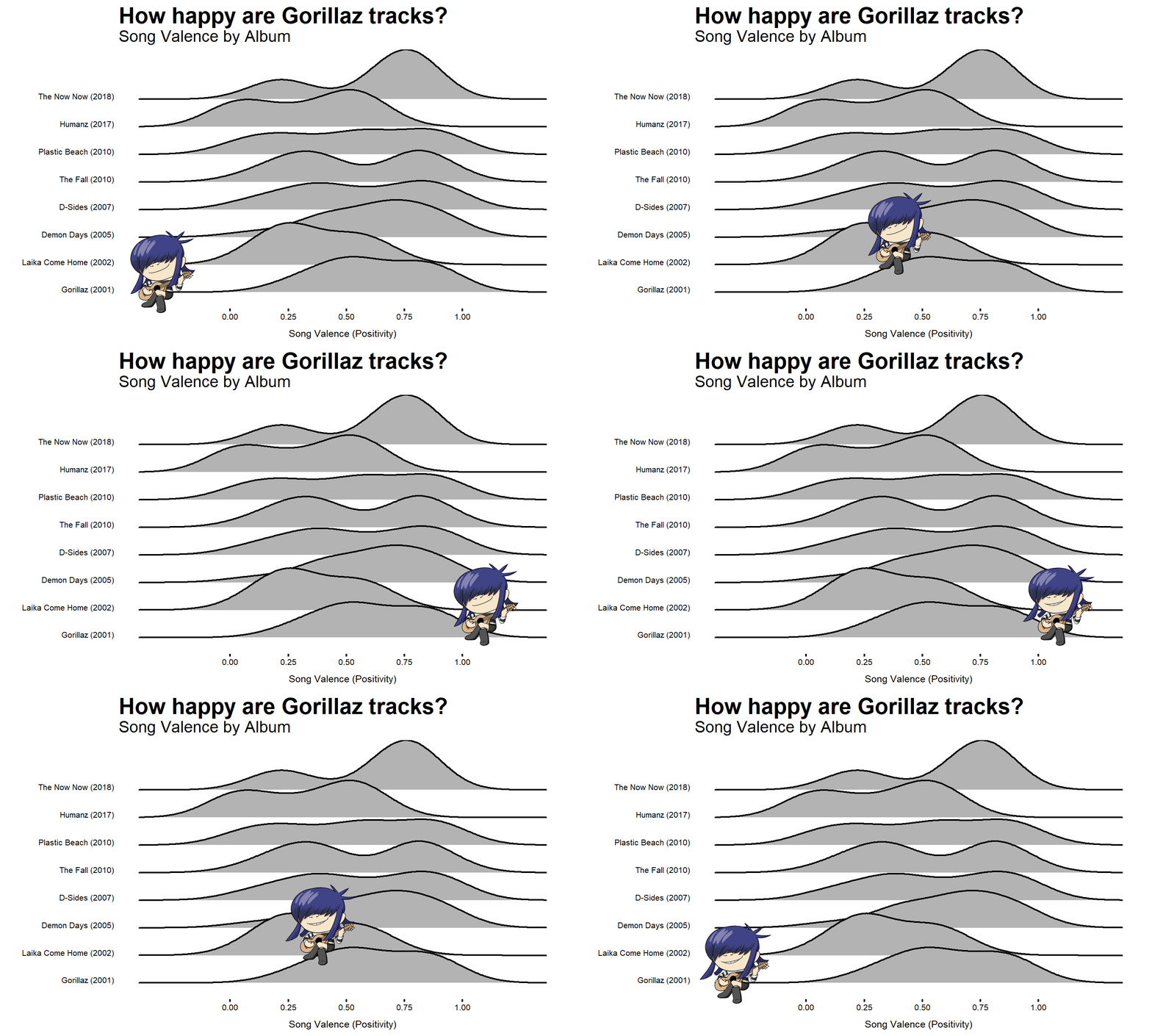
Since the number of frames for the gif was so low, I looped the gif 10
times looped gif. I then added the gif frame by frame with
image_composite(). To move the gif across the axes, I created a vector
of pixel values: x_movement and y_movement.
looped_gif <- c(rep(plot_gif, 10))

frames <- map(1:length(looped_gif), function(frame){
  hjust <- x_movement[frame]
  vjust <- y_movement[frame]
  offset_string <- paste0("+", hjust, "+", vjust)
  image_composite(background, looped_gif[frame], offset = offset_string)
})
Lastly, we used image_animate() with the setting loop = 0 for
infinite looping.
image_animate(image_join(frames), fps = 10, loop = 0)


